A Basic Study Of Broadcasting Using NumPy arrays

Broadcasting is a minor programming idea. It provides the ability to perform arithmetic operations between arrays of different shapes. For this, the shapes of the array must be compatible. It is done by taking advantage of the vectorization concept.

Let’s discuss this idea by example. We can start with element-wise operations

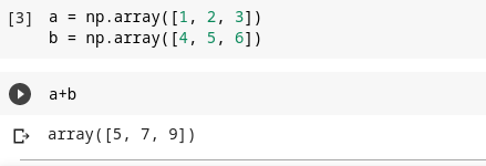
Here a and b are 2 arrays of the same shape. When we add these 2 NumPy arrays together, it adds corresponding elements of these 2 arrays. We call this an element-wise operation. In other words, we don’t want to write a loop. So we can write loop-less code by taking advantage of element-wise operations.

Broadcasting with scalar

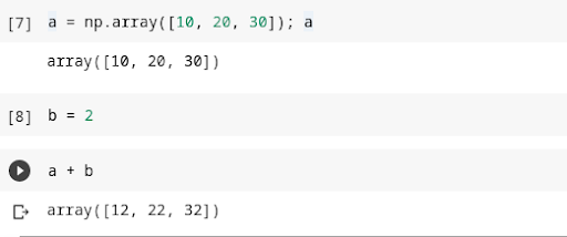
In the above example, a is an array, also called Rank 1 Tensor and b is Rank 0 Tensor or simply a scalar. So we have got these in different ranks. When we say a + b, what happens here is the scalar is stretched into an array so that it can match the shape of a. This is called Broadcasting. Broadcasting means copying 1 or more axes of the tensor to allow it to be the same shape as another Tensor. But it doesn’t really copy.

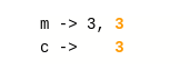
Broadcasting a vector to a matrix

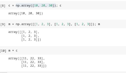
In the above example, we can see the c (Rank 1 Tensor) is copied across the rows of m (Rank 2 Tensor) and thus c is treated as a Rank 2 Tensor. 

Suppose we don’t understand what is happening here, do the following command to understand this concept.

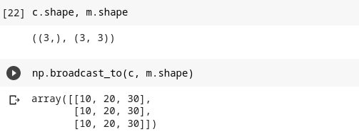
The np.broadcast_to() takes 2 arguments:
The first argument is the array to broadcast and the second is the shape to which it needs to be broadcasted. So in order to perform this operation, the Rank 1 Tensor is broadcasted to a Rank 2 Tensor.

Broadcasting rules

When operating on two arrays, NumPy compares their shapes element-wise. It starts with the trailing dimensions and works its way forward.
2 dimensions are compatible when,

• They are equal
• One of them is one

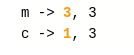
So as per the above example, it starts with the last dimension. Here both m and c have value 3 in the last dimension. So they are compatible.

But in the first dimension c is missing. In this case, we insert 1. When we insert 1, they are compatible as per Rule 2. One of them is 1.

Let’s take another example:

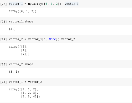
n this example, how do we get this result?
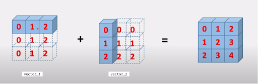
Here both arrays are broadcasted to obtain a common shape (3,3). To make this compatible with broadcasting rules,  the row of vector_1 (1, 3) is duplicated 3 times to match with the row of vector_2 (3, 1) thus producing shape (3, 3) and similarly the column of vector_2  (3, 1)  is broadcasted 3 times to match with columns of vector_1 (1, 3) thus producing shape (3, 3) and then element-wise addition is performed. See the visual representation to understand this idea better.

The goal of broadcasting is to make the tensors have the same shape so we can perform element-wise operations on them. When we normalize datasets during pre-processing for Computer Vision tasks, we need to subtract the mean (scalar) from the dataset (matrix) and divide it by the standard deviation (scalar). For this, we need not write loops over the channels. We can use broadcasting, which vectorizes array operations so that looping occurs in C instead of Python thus increasing the performance. We are here to help you if you would like to work on our resources based on NumPy. Click here to know more.